Direct Link

The PDF version of this tutorial can be found at Google Drive Link.

Acknowledgement

This tutorial is based on slides from this course at NTU Machine Learning 2022 Spring.

2/18 Lecture 1: Introduction of Deep Learning

Preparation 1: ML Basic Concepts

ML is about finding a function.

Besides regression and classification tasks, ML also focuses on Structured Learning – create something with structure (image, document).

Three main ML tasks:

• Regression
• Classification
• Structured Learning

Function with unknown parameters

Guess a function (model) $y=b+wx_1$ (in this case, a linear model) based on domain knowledge. $w$ and $b$ are unknown parameters.

Define Loss From Training Data

Loss is a function itself of parameters, written as $L(b,w)$​.

An example loss function is:

$$ L = \frac{1}{N} \sum_{n} e_n $$

where $e_n$ can be calculated in many ways:

Mean Absolute Error (MAE) $$ e_n = |y_n - \hat{y}_n| $$

Mean Square Error (MSE)

$$ e_n = (y_n - \hat{y}_n)^2 $$

If $y$ and $\hat{y}_n$ are both probability distributions, we can use cross entropy.

Optimization

The goal is to find the best parameter:

$$ w^*, b^* = \arg\min_{w,b} L $$

Solution: Gradient Descent

1. Randomly pick an intitial value $w^0$
2. Compute $\frac{\partial L}{\partial w} \bigg|_{w=w^0}$ (if it’s negative, we should increase $w$; if it’s positive, we should decrease $w$​)
3. Perform update step: $w^1 \leftarrow w^0 - \eta \frac{\partial L}{\partial w} \bigg|_{w=w^0}$ iteratively
4. Stop either when we’ve performed a maximum number of update steps or the update stops ( $\eta \frac{\partial L}{\partial w} = 0$)

If we have two parameters:

1. (Randomly) Pick initial values $w^0, b^0$

2. Compute:

   $w^1 \leftarrow w^0 - \eta \frac{\partial L}{\partial w} \bigg|_{w=w^0, b=b^0}$

   $b^1 \leftarrow b^0 - \eta \frac{\partial L}{\partial b} \bigg|_{w=w^0, b=b^0}$​

Preparation 2: ML Basic Concepts

Beyond Linear Curves: Neural Networks

However, linear models are too simple. Linear models have severe limitations called model bias.

All piecewise linear curves:

More pieces require more blue curves.

How to represent a blue curve (Hard Sigmoid function): Sigmoid function

$$ y = c\cdot \frac{1}{1 + e^{-(b + wx_1)}} = c\cdot \text{sigmoid}(b + wx_1) $$

We can change $w$, $c$ and $b$ to get sigmoid curves with different shapes.

Different Sigmoid curves -> Combine to approximate different piecewise linear functions -> Approximate different continuous functions

From a model with high bias $y=b+wx_1$ to the new model with more features and a much lower bias:

$$ y = b + \sum_{i} c_i \cdot \text{sigmoid}(b_i + w_i x_1) $$

Also, if we consider multiple features $y = b + \sum_{j} w_j x_j$​, the new model can be expanded to look like this:

$$ y = b + \sum_{i} c_i \cdot \text{sigmoid}(b_i + \sum_{j} w_{ij} x_j) $$

Here, $i$ represents each sigmoid function and $j$ represents each feature. $w_{ij}$ represents the weight for $x_j$ that corresponds to the $j$-th feature in the $i$-th sigmoid.

$$ y = b + \boldsymbol{c}^T \sigma(\boldsymbol{b} + W \boldsymbol{x}) $$

$\boldsymbol{\theta}=[\theta_1, \theta_2, \theta_3, ...]^T$ is our parameter vector:

Our loss function is now expressed as $L(\boldsymbol{\theta})$.

Optimization is still the same.

$$ \boldsymbol{\theta}^* = \arg \min_{\boldsymbol{\theta}} L $$

1. (Randomly) pick initial values $\boldsymbol{\theta}^0$​
2. calculate the gradient $\boldsymbol{g} = \begin{bmatrix} \frac{\partial{L}} {\partial{\theta_1}}\bigg|_{\boldsymbol{\theta}=\boldsymbol{\theta}^0} \\ \frac{\partial{L}}{\partial{\theta_2}}\bigg|_{\boldsymbol{\theta}=\boldsymbol{\theta}^0} \\ \vdots \end{bmatrix} = \nabla L(\boldsymbol{\theta}^0)$ with $\boldsymbol{\theta}, \boldsymbol{g} \in \mathbb{R}^n$
3. perform the update step: $\begin{bmatrix} \theta_1^1 \\ \theta_2^1 \\ \vdots \end{bmatrix} \leftarrow \begin{bmatrix} \theta_1^0 \\ \theta_2^0 \\ \vdots \end{bmatrix} - \begin{bmatrix} \eta \frac{\partial{L}}{\partial{\theta_1}}\bigg|_{\boldsymbol{\theta}=\boldsymbol{\theta}^0} \\ \eta \frac{\partial{L}}{\partial{\theta_2}}\bigg|_{\boldsymbol{\theta}=\boldsymbol{\theta}^0} \\ \vdots \end{bmatrix}$, namely $\boldsymbol{\theta}^1 \leftarrow \boldsymbol{\theta}^0 - \eta \boldsymbol{g}$

The terms batch and epoch are different.

$$ \text{num_updates} = \frac{\text{num_examples}}{\text{batch_size}} $$

Batch size $B$​ is also a hyperparameter. One epoch does not tell the number of updates the training process actually has.

More activation functions: RELU

It looks kind of like the Hard Sigmoid function we saw earlier:

As a result, we can use these two RELU curves to simulate the same result as Sigmoid curve.

$$ y = b + \sum_{2i} c_i \max(0, b_i + \sum_j w_{ij}x_j) $$

But, why we want “Deep” network, not “Fat” network? Answer to that will be revealed in a later lecture.

2/25 Lecture 2: What to do if my network fails to train

Preparation 1: ML Tasks

Frameworks of ML

Training data is $\{(\boldsymbol{x}^1, \hat{y}^1), (\boldsymbol{x}^2, \hat{y}^2), ...,(\boldsymbol{x}^N, \hat{y}^N)\}$. Testing data is $\{ \boldsymbol{x}^{N+1}, \boldsymbol{x}^{N+2}, ..., \boldsymbol{x}^{N+M} \}$​

Traing steps:

1. write a function with unknown parameters, namely $y = f_{\boldsymbol{\theta}}(\boldsymbol{x})$​
2. define loss from training data: $L(\boldsymbol{\theta})$
3. optimization: $\boldsymbol{\theta}^* = \arg \min_{\boldsymbol{\theta}} L$​
4. Use $y = f_{\boldsymbol{\theta}^*}(\boldsymbol{x})$​ to label the testing data

General Guide

Potential issues during training

Model bias: the potential function set of our model does not even include the desired optimal function/model.

Large loss doesn’t always imply issues with model bias. There may be issues with optimization. That is, gradient descent does not always produce global minima. We may stuck at a local minima. In the language of function set, the set theoretically contain optimal function $f^*(\boldsymbol{x})$. However, we may never reach that.

Optimization issue

• gain insights from comparison to identify whether the failure of the model is due to optimization issues, overfitting or model bias
• start from shallower networks (or other models like SVM which is much easier to optimize)
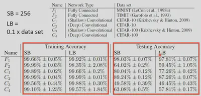
• if deeper networks do not contain smaller loss on training data, then there is optimization issues (as seen from the graph below)

For example, here, the 5-layer should always do better or the same as the 4-layer network. This is clearly due to optimization problems.

Overfitting

Solutions:

• more training data
• data augumentation (in image recognition, it means flipping images or zooming in images)
• use a more constrained model:
  • less parameters
  • sharing parameters
  • less features
  • early stopping
  • regularization
  • dropout

For example, CNN is a more constrained version of the fully-connected vanilla neural network.

Bias-Complexity Trade-off

N-fold Cross Validation

Mismatch

Mismatch occurs when the training dataset and the testing dataset comes from different distributions. Mismatch can not be prevented by simply increasing the training dataset like we did to overfitting. More information on mismatch will be provided in Homework 11.

Preparation 2: Local Minima & Saddle Points

Optimization Failure

Optimization fails not always because of we stuck at local minima. We may also encounter saddle points, which are not local minima but have a gradient of $0$.

All the points that have a gradient of $0$ are called critical points. So, we can’t say that our gradient descent algorithms always stops because we stuck at local minima – we may stuck at saddle points as well. The correct way to say is that gradient descent stops when we stuck at a critical point.

If we are stuck at a local minima, then there’s no way to further decrease the loss (all the points around local minima are higher); if we are stuck at a saddle point, we can escape the saddle point. But, how can we differentiate a saddle point and local minima?

Identify which kinds of Critical Points

$L(\boldsymbol{\theta})$ around $\boldsymbol{\theta} = \boldsymbol{\theta}'$ can be approximated (Taylor Series)below:

$$ L(\boldsymbol{\theta}) \approx L(\boldsymbol{\theta}') + (\boldsymbol{\theta} - \boldsymbol{\theta}')^T \boldsymbol{g} + \frac{1}{2} (\boldsymbol{\theta} - \boldsymbol{\theta}')^T H (\boldsymbol{\theta} - \boldsymbol{\theta}') $$

Gradient $\boldsymbol{g}$ is a vector:

$$ \boldsymbol{g} = \nabla L(\boldsymbol{\theta}') $$ $$ \boldsymbol{g}_i = \frac{\partial L(\boldsymbol{\theta}')}{\partial \boldsymbol{\theta}_i} $$

Hessian $H$ is a matrix:

$$ H_{ij} = \frac{\partial^2}{\partial \boldsymbol{\theta}_i \partial \boldsymbol{\theta}_j} L(\boldsymbol{\theta}') $$

The green part is the Gradient and the red part is the Hessian.

When we are at the critical point, The approximation is “dominated” by the Hessian term.

Namely, our approximation formula becomes:

$$ L(\boldsymbol{\theta}) \approx L(\boldsymbol{\theta}') + \frac{1}{2} (\boldsymbol{\theta} - \boldsymbol{\theta}')^T H (\boldsymbol{\theta} - \boldsymbol{\theta}') = L(\boldsymbol{\theta}') + \frac{1}{2} \boldsymbol{v}^T H \boldsymbol{v} $$

Local minima:

• For all $\boldsymbol{v}$, if $\boldsymbol{v}^T H \boldsymbol{v} > 0$ ( $H$ is positive definite, so all eigenvalues are positive), around $\boldsymbol{\theta}'$: $L(\boldsymbol{\theta}) > L(\boldsymbol{\theta}')$​

Local maxima:

• For all $\boldsymbol{v}$, if $\boldsymbol{v}^T H \boldsymbol{v} < 0$ ( $H$ is negative definite, so all eigenvalues are negative), around $\boldsymbol{\theta}'$: $L(\boldsymbol{\theta}) < L(\boldsymbol{\theta}')$

Saddle point:

• Sometimes $\boldsymbol{v}^T H \boldsymbol{v} < 0$, sometimes $\boldsymbol{v}^T H \boldsymbol{v} > 0$. Namely, $H$​ is indefinite – some eigenvalues are positive and some eigenvalues are negative.

Example:

Escaping saddle point

If by analyzing $H$’s properpty, we realize that it’s indefinite (we are at a saddle point). We can also analyze $H$ to get a sense of the parameter update direction!

Suppose $\boldsymbol{u}$ is an eigenvector of $H$ and $\lambda$ is the eigenvalue of $\boldsymbol{u}$.

$$ \boldsymbol{u}^T H \boldsymbol{u} = \boldsymbol{u}^T (H \boldsymbol{u}) = \boldsymbol{u}^T (\lambda \boldsymbol{u}) = \lambda (\boldsymbol{u}^T \boldsymbol{u}) = \lambda \|\boldsymbol{u}\|^2 $$

If the eigenvalue $\lambda < 0$, then $\boldsymbol{u}^T H \boldsymbol{u} = \lambda \|\boldsymbol{u}\|^2 < 0$ (eigenvector $\boldsymbol{u}$ can’t be $\boldsymbol{0}$). Because $L(\boldsymbol{\theta}) \approx L(\boldsymbol{\theta}') + \frac{1}{2} \boldsymbol{u}^T H \boldsymbol{u}$, we know $L(\boldsymbol{\theta}) < L(\boldsymbol{\theta}')$. By definition, $\boldsymbol{\theta} - \boldsymbol{\theta}' = \boldsymbol{u}$. If we perform $\boldsymbol{\theta} = \boldsymbol{\theta}' + \boldsymbol{u}$, we can effectively decrease $L$. We can escape the saddle point and decrease the loss.

However, this method is seldom used in practice because of the huge computation need to compute the Hessian matrix and the eigenvectors/eigenvalues.

Local minima v.s. saddle point

A local minima in lower-dimensional space may be a saddle point in a higher-dimension space. Empirically, when we have lots of parameters, local minima is very rare.

Preparation 3: Batch & Momentum

Small Batch v.s. Large Batch

Note that here, “time for cooldown” does not always determine the time it takes to complete an epoch.

Emprically, large batch size $B$​ does not require longer time to compute gradient because of GPU’s parallel computing, unless the batch size is too big.

Smaller batch requires longer time for one epoch (longer time for seeing all data once).

However, large batches are not always better than small batches. That is, the noise brought by small batches lead to better performance (optimization).

Small batch is also better on testing data (overfitting).

This may be because that large batch is more likely to lead to us stucking at a sharp minima, which is not good for testing loss. Because of noises, small batch is more likely to help us escape sharp minima. Instead, at convergence, we will more likely end up in a flat minima.

Batch size is another hyperparameter.

Momentum

Vanilla Gradient Descent:

Gradient Descent with Momentum:

Concluding Remarks

Preparation 4: Learning Rate

Problems with Gradient Descent

The fact that training process is stuck does not always mean small gradient.

Training can be difficult even without critical points. Gradient descent can fail to send us to the global minima even under the circumstance of a convex error surface. You can’t fix this problem by adjusting the learning rate $\eta$.

Learning rate can not be one-size-fits-all. If we are at a place where the gradient is high (steep surface), we expect $\eta$ to be small so that we don’t overstep; if we are at a place where the gradient is small (flat surface), we expect $\eta$ to be large so that we don’t get stuck at one place.

Adagrad

Formulation for one parameter:

$$ \boldsymbol{\theta}_i^{t+1} \leftarrow \boldsymbol{\theta}_i^{t} - \eta \boldsymbol{g}_i^t $$ $$ \boldsymbol{g}_i^t = \frac{\partial L}{\partial \boldsymbol{\theta}_i} \bigg |_{\boldsymbol{\theta} = \boldsymbol{\theta}^t} $$

The new formulation becomes:

$$ \boldsymbol{\theta}_i^{t+1} \leftarrow \boldsymbol{\theta}_i^{t} - \frac{\eta}{\sigma_i^t} \boldsymbol{g}_i^t $$

$\sigma_i^t$ is both parameter-dependent ( $i$) and iteration-dependent ( $t$). It is called Root Mean Square. It is used in Adagrad algorithm.

$$ \sigma_i^t = \sqrt{\frac{1}{t+1} \sum_{i=0}^t (\boldsymbol{g}_i^t)^2} $$

Why this formulation works?

RMSProp

However, this formulation still has some problems. We assumed that the gradient for one parameter will stay relatively the same. However, it’s not always the case. For example, there may be places where the gradient becomes large and places where the gradient becomes small (as seen from the graph below). The reaction of this formulation to a new gradient change is very slow.

The new formulation is now:

$$ \sigma_i^t = \sqrt{\alpha(\sigma_i^{t-1})^2 + (1-\alpha)(\boldsymbol{g}_i^t)^2} $$ $\alpha$ is a hyperparameter ( $0 < \alpha < 1$). It controls how important the previously-calculated gradient is.

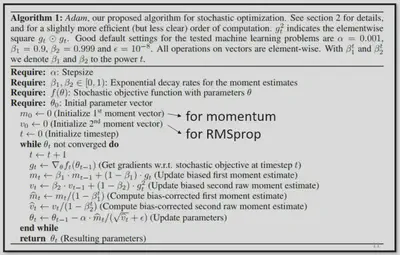
Adam

The Adam optimizer is basically the combination of RMSProp and Momentum.

Learning Rate Scheduling

This is the optimization process with Adagrad:

To prevent the osciallations at the final stage, we can use two methods:

$$ \boldsymbol{\theta}_i^{t+1} \leftarrow \boldsymbol{\theta}_i^{t} - \frac{\eta^t}{\sigma_i^t} \boldsymbol{g}_i^t $$

Learning Rate Decay

As the training goes, we are closer to the destination. So, we reduce the learning rate $\eta^t$​.

This improves the previous result:

Warm up

We first increase $\eta ^ t$ and then decrease it. This method is used in both the Residual Network and Transformer paper. At the beginning, the estimate of $\sigma_i^t$​​ has large variance. We can learn more about this method in the RAdam paper.

Summary

Preparation 5: Loss

How to represent classification

We can’t directly apply regression to classification problems because regression tends to penalize the examples that are “too correct.”

It’s also problematic to directly represent Class 1 as numeric value $1$, Class 2 as $2$, Class 3 as $3$​. That is, this representation has an underlying assumption that Class 1 is “closer” or more “similar” to Class 2 than Class 3. However, this is not always the case.

One possible model is:

$$ f(x) = \begin{cases} 1 & g(x) > 0 \\ 2 & \text{else} \end{cases} $$

The loss function denotes the number of times $f$ gets incorrect results on training data.

$$ L(f) = \sum_n \delta(f(x^n) \neq \hat{y}^n) $$

We can represent classes as one-hot vectors. For example, we can represent Class $1$ as $\hat{y} = \begin{bmatrix} 1 \ 0 \ 0 \end{bmatrix} $, Class $2 $ as $\hat{y} = \begin{bmatrix} 0 \ 1 \ 0 \end{bmatrix} $ and Class $3 $ as $\hat{y} = \begin{bmatrix} 0 \ 0 \ 1 \end{bmatrix}$.

Softmax

$$ y_i' = \frac{\exp(y_i)}{\sum_j \exp(y_j)} $$

We know that $0 < y_i' < 1$ and $\sum_i y_i' = 1$.

Loss of Classification

Mean Squared Error (MSE)

$$ e = \sum_i (\boldsymbol{\hat{y}}_i - \boldsymbol{y}_i')^2 $$

Cross-Entropy

$$ e = -\sum_i \boldsymbol{\hat{y}}_i \ln{\boldsymbol{y}_i'} $$

Minimizing cross-entropy is equivalent to maximizing likelihood.

Cross-entropy is more frequently used for classification than MSE. At the region with higher loss, the gradient of MSE is close to $0$. This is not good for gradient descent.

Generative Models

$$ P(C_1 \mid x) = \frac{P(C_1, x)}{P(x)} = \frac{P(x \mid C_1)P(C_1)}{P(x \mid C_1)P(C_1) + P(x \mid C_2)P(C_2)} $$

We can therefore predict the distribution of $x$:

$$ P(x) = P(x \mid C_1)P(C_1) + P(x \mid C_2)P(C_2) $$

Prior

$P(C_1)$ and $P(C_2)$ are called prior probabilities.

Gaussian distribution

$$ f_{\mu, \Sigma}(x) = \frac{1}{(2\pi)^{D/2} |\Sigma|^{1/2}} \exp\left(-\frac{1}{2} (x - \mu)^T \Sigma^{-1} (x - \mu)\right) $$

Input: vector $x$, output: probability of sampling $x$. The shape of the function determines by mean $\mu$ and covariance matrix $\Sigma$. ==Technically, the output is the probability density, not exactly the probability, through they are positively correlated.==

Maximum Likelihood

We assume $x^1, x^2, x^3, \cdots, x^{79}$ generate from the Gaussian ( $\mu^*, \Sigma^*$) with the maximum likelihood.

$$ L(\mu, \Sigma) = f_{\mu, \Sigma}(x^1) f_{\mu, \Sigma}(x^2) f_{\mu, \Sigma}(x^3) \cdots f_{\mu, \Sigma}(x^{79}) $$ $$ \mu^*, \Sigma^* = \arg \max_{\mu,\Sigma} L(\mu, \Sigma) $$

The solution is as follows:

$$ \mu^* = \frac{1}{79} \sum_{n=1}^{79} x^n $$ $$ \Sigma^* = \frac{1}{79} \sum_{n=1}^{79} (x^n - \mu^*)(x^n - \mu^*)^T $$

But the above generative model fails to give a high-accuracy result. Why? In that formulation, every class has its unique mean vector and covariance matrix. The size of the covariance matrix tends to increase as the feature size of the input increases. This increases the number of trainable parameters, which tends to result in overfitting. Therefore, we can force different distributions to share the same covariance matrix.

Intuitively, the new covariance matrix is the sum of the original covariance matrices weighted by the frequencies of samples in each distribution.

Three steps to a probability distribution model

We can always use whatever distribution we like (we use Guassian in the previous example).

If we assume all the dimensions are independent, then you are using Naive Bayes Classifier.

$$ P(\boldsymbol{x} \mid C_1) = P(\begin{bmatrix}x_1 \\ x_2 \\ \vdots \\ x_K \end{bmatrix} \mid C_1) = P(x_1 \mid C_1)P(x_2 \mid C_1) \dots P(x_K \mid C_1) $$

Each $P(x_m \mid C_1)$ is now a 1-D Gaussian. For binary features, you may assume they are from Bernouli distributions.

But if the assumption does not hold, the Naive Bayes Classifier may have a very high bias.

Posterior Probability

$$ \begin{align} P(C_1 | x) &= \frac{P(x | C_1) P(C_1)}{P(x | C_1) P(C_1) + P(x | C_2) P(C_2)} \\ &= \frac{1}{1 + \frac{P(x | C_2) P(C_2)}{P(x | C_1) P(C_1)}} \\ &= \frac{1}{1 + \exp(-z)} \\ &= \sigma(z) \\ \end{align} $$ $$ \begin{align} z &= \ln \frac{P(x | C_1) P(C_1)}{P(x | C_2) P(C_2)} \\ &= \ln \frac{P(x | C_1)}{P(x | C_2)} + \ln \frac{P(C_1)}{P(C_2)} \\ &= \ln \frac{P(x | C_1)}{P(x | C_2)} + \ln \frac{\frac{N_1}{N_1+N_2}}{\frac{N_2}{N_1+N_2}} \\ &= \ln \frac{P(x | C_1)}{P(x | C_2)} + \ln \frac{N_1}{N_2} \\ \end{align} $$

Furthermore:

$$ \begin{align} \ln \frac{P(x | C_1)}{P(x | C_2)} &= \ln \frac{\frac{1}{(2\pi)^{D/2} |\Sigma_1|^{1/2}} \exp\left\{-\frac{1}{2} (x - \mu^1)^T \Sigma_1^{-1} (x - \mu^1)\right\}} {\frac{1}{(2\pi)^{D/2} |\Sigma_2|^{1/2}} \exp\left\{-\frac{1}{2} (x - \mu^2)^T \Sigma_2^{-1} (x - \mu^2)\right\}} \\ &= \ln \frac{|\Sigma_2|^{1/2}}{|\Sigma_1|^{1/2}} \exp \left\{ -\frac{1}{2} [(x - \mu^1)^T \Sigma_1^{-1} (x - \mu^1)-\frac{1}{2} (x - \mu^2)^T \Sigma_2^{-1} (x - \mu^2)] \right\} \\ &= \ln \frac{|\Sigma_2|^{1/2}}{|\Sigma_1|^{1/2}} - \frac{1}{2} \left[(x - \mu^1)^T \Sigma_1^{-1} (x - \mu^1) - (x - \mu^2)^T \Sigma_2^{-1} (x - \mu^2)\right] \end{align} $$

Further simplification goes:

Since we assume the distributions share the covariance matrix, we can further simplify the formula:

$$ P(C_1 \mid x) = \sigma(w^Tx + b) $$

This is why the decision boundary is a linear line.

In generative models, we estimate $N_1, N_2, \mu^1, \mu^2, \Sigma$, then we have $\boldsymbol{w}$ and $b$. How about directly find $\boldsymbol{w}$ and $b$​?

Logistic Regression

We want to find $P_{w,b}(C_1 \mid x)$. If $P_{w,b}(C_1 \mid x) \geq 0.5$, output $C_1$. Otherwise, output $C_2$.

$$ P_{w,b}(C_1 \mid x) = \sigma(z) = \sigma(w \cdot x + b) = \sigma(\sum_i w_ix_i + b) $$

The function set is therefore (including all different $w$ and $b$):

$$ f_{w,b}(x) = P_{w,b}(C_1 \mid x) $$

Given the training data $\{(x^1, C_1),(x^2, C_1),(x^3, C_2),\dots, (x^N, C_1)\}$, assume the data is generated based on $f_{w,b}(x) = P_{w,b}(C_1 \mid x)$. Given a set of $w$ and $b$, the probability of generating the data is:

$$ L(w,b) = f_{w,b}(x^1)f_{w,b}(x^2)\left(1-f_{w,b}(x^3)\right)...f_{w,b}(x^N) $$ $$ w^*,b^* = \arg \max_{w,b} L(w,b) $$

We can write the formulation by introducing $\hat{y}^i$, where:

$$ \hat{y}^i = \begin{cases} 1 & x^i \text{ belongs to } C_1 \\ 0 & x^i \text{ belongs to } C_2 \end{cases} $$ $$ C(p,q) = - \sum_x p(x) \ln \left( q(x) \right) $$

Therefore, minimizing $- \ln L(w,b)$ is actually minimizing the cross entropy between two distributions: the output of function $f_{w,b}$ and the target $\hat{y}^n$​​.

$$ L(f) = \sum_n C(f(x^n), \hat{y}^n) $$ $$ C(f(x^n), \hat{y}^n) = -[\hat{y}^n \ln f(x^n) + (1-\hat{y}^n) \ln \left(1-f(x^n)\right)] $$

Here, the larger the difference ( $\hat{y}^n - f_{w,b}(x^n)$) is, the larger the update.

Therefore, the update step for logistic regression is:

$$ w_i \leftarrow w_i - \eta \sum_n - \left(\hat{y}^n - f_{w,b}(x^n)\right)x_i^n $$

This looks the same as the update step for linear regression. However, in logistic regression, $f_{w,b}, \hat{y}^n \in \{0,1\}$.

Comparision of the two algorithms:

Why using square error instead of cross entropy on logistic regression is a bad idea?

In either case, this algorithm fails to produce effective optimization. A visualization of the loss functions for both cross entropy and square error is illustrated below:

Discriminative v.s. Generative

The logistic regression is an example of discriminative model, while the Gaussian posterior probability method is an example of generative model, through their function set is the same.

We will not obtain the same set of $w$ and $b$. The same model (function set) but different function is selected by the same training data. The discriminative model tends to have a better performance than the generative model.

A toy example shows why the generative model tends to perform less well. We assume Naive Bayes here, namely $P(x \mid C_i) = P(x_1 \mid C_i)P(x_2 \mid C_i)$ if $x \in \mathbb{R}^2$. The result is counterintuitive – we expect the testing data to be classified as Class 1 instead of Class 2.

Multiclass Classification

Softmax will further enhance the maximum $z$ input, expanding the difference between a large value and a small value. Softmax is an approximation of the posterior probability. If we assume the previous Gaussian generative model that share the same covariance matrix amongst distributions, we can derive the exact same Softmax formulation. We can also derive Softmax from maximum entropy (similar to logistic regression).

Like the binary classification case earlier, the multiclass classification aims to maximize likelihood, which is the same as minimizing cross entropy.

Limitations of Logistic Regression

Solution: feature transformation

However, it is not always easy to find a good transformation. We can cascade logistic regression models.

Preparation 6: Batch Normalization

In a linear model, when the value at each dimension have very distinct values, we may witness an error surface that is steep in one dimension and smooth in the other, as seen from the left graph below. If we can restrict the value at each dimension to be of the same range, we can make the error surface more “trainable,” as seen from the right graph below.

Feature Normalization

Recall standardization: $$ \boldsymbol{\tilde{x}}^{r}_{i} \leftarrow \frac{\boldsymbol{x}^{r}_{i} - m_{i}}{\sigma_{i}} $$ $i$ represents the dimension of the vector $\boldsymbol{x}$ and $r$ represents the index of the datapoint.

For the Sigmoid activation function, we can apply feature normalization on $\boldsymbol{z}$ (before Sigmoid) so that all the values are concentrated close to $0$. But in other cases, it’s acceptable to apply feature normalization on either $\boldsymbol{z}$ or $\boldsymbol{a}$.

When doing feature normalization, we can use element-wise operation on $\boldsymbol{z}$.

Batch Normalization Training

Notice that now if $\boldsymbol{z}^1$ changes, $\boldsymbol{\mu}, \boldsymbol{\sigma}, \boldsymbol{\tilde{z}}^1, \boldsymbol{\tilde{z}}^2, \boldsymbol{\tilde{z}}^3$​ will all change. That is, the network is now considering all the inputs and output a bunch of outputs. This could be slow and memory-intensive because we need to load the entire dataset. So, we consider batches – Batch Normalization.

We can also make a small improvement:

$$ \boldsymbol{\hat{z}}^{i} = \boldsymbol{\gamma} \odot \boldsymbol{\tilde{z}}^{i} + \boldsymbol{\beta} $$ We set $\boldsymbol{\gamma}$ to $[1,1,...]^T$ and $\boldsymbol{\beta}$ to $[0,0,...]^T$​ at the start of the iteration (they are *parameters* of the network). This means that the range will still the the same amongst different dimensions in the beginning. As the training goes, we may want to lift the contraint that each dimension has a mean of 0.

Batch Normalization Testing/Inference

We do not always have batch at testing stage.

Computing the moving average of $\boldsymbol{\mu}$ and $\boldsymbol{\sigma}$​ of the batches during training (PyTorch has an implementation of this). The hyperparamteer $p$ is usually $0.1$. $\boldsymbol{\mu^t}$ is the $t$-th batch’s $\boldsymbol{\mu}$. $$ \boldsymbol{\bar{\mu}} \leftarrow p \boldsymbol{\bar{\mu}} + (1-p) \boldsymbol{\mu^t} $$

3/04 Lecture 3: Image as input

Preparation 1: CNN

CNN

A neuron does not have to see the whole image. Every receptive field has a set of neurons (e.g. 64 neurons).

The same patterns appear in different regions. Every receptive field has the neurons with the same set of parameters.

The convolutional layer produces a feature map.

The feature map becomes a “new image.” Each filter convolves over the input image.

A filter of size 3x3 will not cause the problem of missing “large patterns.” This is because that as we go deeper into the network, our filter will read broader information (as seen from the illustration below).

Subsampling the pixels will not change the object. Therefore, we always apply Max Pooling (or other methods) after convolution to reduce the computation cost.

Limitations of CNN

CNN is not invariant to scaling and rotation (we need data augumentation).

3/11 Lecture 4: Sequence as input

Preparation 1: Self-Attention

Vector Set as Input

We often use word embedding for sentences. Each word is a vector, and therefore the whole sentence is a vector set.

Audio can also be represented as a vector set. We often use a vector to represent a $25ms$-long audio.

Graph is also a set of vectors (consider each node as a vector of various feature dimensions).

Output

Each vector has a label (e.g. POS tagging). This is also called sequence labeling.

The whole sequence has a label (e.g. sentiment analysis).

It is also possible that the model has to decide the number of labels itself (e.g. translation). This is also called seq2seq.

Sequence Labeling

The self-attention module will try to consider the whole sequence and find the relevant vectors within the sequence (based on the attention score $\alpha$ for each pair).

There are many ways to calculate $\alpha$:

Additive:

Dot-product: (the most popular method)

The attention score will then pass through softmax (not necessary, RELU is also possible).

$$ \alpha_{1,i}' = \frac{\exp(\alpha_{1,i})}{\sum_j \exp(\alpha_{1,j})} $$

We will then extract information based on attention scores (after applying softmax).

$$ \boldsymbol{b}^1 = \sum_i \alpha_{1,i}' \boldsymbol{v}^i $$

If $\boldsymbol{a}^1$ is most similar to $\boldsymbol{a}^2$, then $\alpha_{1,2}'$ will be the highest. Therefore, $\boldsymbol{b}^1$ will be dominated by $\boldsymbol{a}^2$.

Preparation 2: Self-Attention

Review

The creation of $\boldsymbol{b}^n$ is in parallel. We don’t wait.

Matrix Form

We can also view self-attention using matrix algebra.

Since every $\boldsymbol{a}^n$ will produce $\boldsymbol{q}^n, \boldsymbol{k}^n, \boldsymbol{v}^n$​, we can write the process in matrix-matrix multiplication form.

Remeber that:

As a result, we can write:

In addition, we can use the same method for calculating attention scores:

Here, since $K = [\boldsymbol{k}^1, \boldsymbol{k}^2, \boldsymbol{k}^3, \boldsymbol{k}^4]$​, we use its transpose $K^T$.

By applying softmax, we make sure that every column of $A'$ sum up to $1$, namely, for $i\in\{1,2,3,4\}$, $\sum_j \alpha_{i,j}' = 1$​​.

We use the same method to write the final output $\boldsymbol{b}^n$:

This is based on matrix-vector rules:

Summary of self-attention: the process from $I$ to $O$

Multi-Head Self-Attention

We may have different metrics of relevance. As a result, we may consider multi-head self-attention, a variant of self-attention.

We can then combine $\boldsymbol{b}^{i,1}, \boldsymbol{b}^{i,2}$ to get the final $\boldsymbol{b}^i$.

Positional Encoding

Self-attention does not care about position information. For example, it does not care whether $\boldsymbol{a}^1$ is close to $\boldsymbol{a}^2$ or $\boldsymbol{a}^4$. To solve that, we can apply positional encoding. Each position has a unique hand-crafted positional vector $\boldsymbol{e}^i$. We then apply $\boldsymbol{a}^i \leftarrow \boldsymbol{a}^i + \boldsymbol{e}^i$​​.

Speech

If the input sequence is of length $L$, the attention matrix $A'$ is a matrix of $L$x $L$​, which may require a large amount of computation. Therefore, in practice, we don’t look at the whole audio sequence. Instead, we use truncated self-attention, which only looks at a small range.

Images

What’s its difference with CNN?

• CNN is the self-attention that can only attends in a receptive field. Self-attention is a CNN with learnable receptive field.
• CNN is simplified self-attention. Self-attention is the complex version of CNN.

Self-attention is more flexible and therefore more prune to overfitting if the dataset is not large enough. We can also use conformer, a combination of the two.

Self-Attention v.s. RNN

Self-attention is a more complex version of RNN. RNN can be bi-directional, so it is possible to consider the whole input sequence like self-attention. However, it struggles at keeping a vector at the start of the sequence in the memory. It’s also computationally-expensive because of its sequential (non-parallel) nature.

Graphs

This is one type of GNN.

Extra Material: RNN

How to represent a word?

1-of-N Encoding

The vector is lexicon size. Each dimension corresponds to a word in the lexicon. The dimension for the word is 1, and others are 0. For example, lexicon = {apple, bag, cat, dog, elephant}. Then, apple = [1 0 0 0 0].

RNN architecture

The memory units must have an initial value. Changing the order of the sequence will change the output.

The same network is used again and again. If the words before a particular word is different, then the values stored in the memory will be different, therefore causing the probability (i.e. output) of the same word different.

We can also make the RNN deeper:

Elman & Jordan Network

Jordan Network tends to have a better performance because we can know what exactly is in the memory unit (the output itself).

Bidirectional RNN

We can also train two networks at once. This way, the network can consider the entire input sequence.

Long Short-Term Memory (LSTM)

$4$ inputs: input, signal to Input Gate, signal to Output Gate, signal to Forget Gate

Why LSTM? The RNN will wipe out memory in every new timestamp, therefore having a really short short-term memory. However, the LSTM can hold on to the memory as long as the Forget Gate $f(z_f)$ is $1$​.

This is the structure of a LSTM cell/neuron:

When $f(z_f)=1$, memory $c$ is completely remembered; when $f(z_f)=0$, memory $c$ is completely forgotten (since $c \cdot f(z_f)=0$​).

When $f(z_i)=1$, input $g(z)$ is completely passed through; when $f(z_i)=0$, $g(z)$ is blocked.

Same story for $f(z_o)$.

Multi-Layer LSTM

A LSTM neuron has four times more parameters than a vanilla neural network neuron. In vanilla neural network, every neuron is a function mapping a input vector to a output scalar. In LSTM, the neuron maps $4$ inputs to $1$ output.

Assume the total number of cells is $n$.

We will apply $4$ linear transformations to get $\boldsymbol{z^f, z^i, z, z^o}$. Each of them represents a type of input to the LSTM neuron. Each of them is a vector in $\mathbb{R}^n$. The $i$-th entry is the input to the $i$​​​-th neuron.

We can use element-wise operations on those vectors to conduct these operations for all $n$ cells at the same time. In addition, the $z$ inputs are based on not only the current input $\boldsymbol{x^t}$, but also the memory cell $\boldsymbol{c^{t-1}}$ and the previous output $\boldsymbol{h^{t-1}}$.

RNN Training

RNN training relies on Backpropagation Through Time (BPTT), a variant of backpropagation. RNN-based network is not always easy to learn.

This is why it is difficult to train RNN. When we are at the flat plane, we often have a large learning rate. If we happen to step on the edge of the steep cliff, we may jump really far (because of the high learning rate and high gradient). This may cause optimization failure and segmentation fault.

This can be solved using Clipping. We can set a maximum threshold for the gradient, so that it does not become really high.

Why do we observe this kind of behavior for RNN’s error surface?

We can notice that the same weight $w$ is applied many times in different time. This causes the problem because any change in $w$ will either has not effect on the final output $y^N$ or a huge impact.

One solution is LSTM. It can deal with gradient vanishing, but not gradient explode. As a result, most points on LSTM error surface with have a high gradient. When training LSTM, we can thus set the learning rate a relatively small value.

Why LSTM solves gradient vanishing? Memory and input are added. The influence never disappears unless Forget Gate is closed.

An alternative option is Gated Recurrent Unit (GRU). It is simpler than LSTM. It only has 2 gates: combining the Forget Gate and the Input Gate.

More Applications

RNN can also be applied on many-to-one tasks (input is a vector sequence, but output is only one output), such as sentiment analysis. We can set the output of RNN at the last timestamp as our final output.

RNN can be used on many-to-many tasks (both input and output are vector sequences, but the output is shorter). For example, when doing speech recognition task, we can use Connectionist Temporal Classification (CTC).

RNN can also be applied on sequence-to-sequence learning (both input and output are both sequences with different lengths), such as machine translation.

Extra Material: GNN

How do we utilize the structures and relationship to help train our model?

Spatial-Based Convolution

• Aggregation: use neighbor features to update hidden states in the next layer
• Readout: use features of all the nodes to represent the whole graph $h_G$​

NN4G (Neural Network for Graph)

$$ h_3^0 = \boldsymbol{w}_0 \cdot \boldsymbol{x}_3 $$ $$ h_3^1 = \hat{w}_{1,3}(h_0^0 + h_2^0 + h_4^0) + \boldsymbol{w}_1 \cdot \boldsymbol{x}_3 $$

DCNN (Diffusion-Convolution Neural Network)

$$ h_3^0 = w_3^0 MEAN(d(3,\cdot)=1) $$ $$ h_3^1 = w_3^1 MEAN(d(3,\cdot)=2) $$

Node features:

3/18 Lecture 5: Sequence to sequence

Preparation 1 & 2: Transformer

Roles

We input a sequence and the model output a sequence. The output length is determined by the model. We use it for speech recognition and translation.

Seq2seq is widely used for QA tasks. Most NLP applications can be viewed as QA tasks. However, we oftentimes use specialized models for different NLP applications.

Seq2seq can also be used on multi-label classification (an object can belong to multiple classes). This is different from multi-class classification, in which we need to classify an object into one class out of many classes.

The basic components of seq2seq is:

Encoder

We need to output a sequence that has the same length as the input sequence. We can technically use CNN or RNN to accomplish this. In Transformer, they use self-attention.

The state-of-the-art encoder architecture looks like this:

The Transformer architecture looks like this:

Residual connection is a very popular technique in deep learning: $\text{output}_{\text{final}} = \text{output} + \text{input}$

Decoder

Autoregressive (AT)

Decoder will receive input that is the its own output in the last timestamp. If the decoder made a mistake in the last timestamp, it will continue that mistake. This may cause error propagation.

The encoder and the decoder of the Transformer is actually quite similar if we hide one part of the decoder.

Masked self-attention: When considering $\boldsymbol{b}^i$, we will only take into account $\boldsymbol{k}^j$, $j \in [0,i)$. This is because the decoder does not read the input sequence all at once. Instead, the input token is generated one after another.

We also want to add a stop token (along with the vocabulary and the start token) to give the decoder a mechanism that it can control the length of the output sequence.

Non-autoregressive (NAT)

How to decide the output length for NAT decoder?

• Another predictor for output length.
• Determine a maximum possible length of sequence, $n$. Feed the decoder with $n$​ START tokens. Output a very long sequence, ignore tokens after END.

Advantage: parallel (relying on self-attention), more stable generation (e.g., TTS) – we can control the output-length classifier to manage the length of output sequence

NAT is usually worse than AT because of multi-modality.

Encoder-Decoder

Cross Attention:

$\alpha_i'$ is the attention score after softmax:

Training

This is very similar to how to we train a classification model. Every time the model creates an output, the model makes a classification.

Our goal is to minimize the sum of cross entropy of all the outputs.

Teacher forcing: using the ground truth as input.

Copy Mechanism

Sometimes we may want the model to just copy the input token. For example, consider a chatbot, when the user inputs “Hi, I’m ___,” we don’t expect the model to generate an output of the user’s name because it’s not likely in our training set. Instead, we want the model to learn the pattern: when it sees input “I’m [some name],” it can output “Hi [some name]. Nice to meet you!”

Guided Attention

In some tasks, input and output are monotonically aligned. For example, speech recognition, TTS (text-to-speech), etc. We don’t want the model to miass some important portions of the input sequence in those tasks.

We want to force the model to learn a particular order of attention.

• monotonic attention
• location-aware attention

Beam Search

The red path is greedy decoding. However, if we give up a little bit at the start, we may get a better global optimal path. In this case, the green path is the best one.

We can use beam search to find a heuristic.

However, sometimes randomness is needed for decoder when generating sequence in some tasks (e.g. sentence completion, TTS). In those tasks, finding a “good path” may not be the best thing because there’s no correct answer and we want the model to be “creative.” In contrast, beam search may be more beneficial to tasks like speech recognition.

Scheduled Sampling

At training, the model always sees the “ground truth” – correct input sequence. At testing, the model is fed with its own output in the previous round. This may cause the model to underperform because it may never see a “wrong input sequence” before (exposure bias). Therefore, we may want to train the model with some wrong input sequences. This is called Scheduled Sampling. But this may hurt the parallel capability of the Transformer.

3/25 Lecture 6: Generation

Preparation 1: GAN Basic Concepts

Generator is a network that can output a distribution.

Why we bother add a distribution into our network?

In this video game frame prediction example, the model is trained on a dataset of two coexisting possibilities – the role turning left and right. As a result, the vanilla network will seek to balance the two. Therefore, it could create a frame that a role splits into two: one turning left and one turning right.

This causes problems. Therefore, we want to add a distribution into the network. By doing so, the output of the network will also become a distribution itself. We especially prefer this type of network when our tasks need “creativity.” The same input has different correct outputs.

Unconditional Generation

For unconditional generation, we don’t need the input $x$.

GAN architecture also has a discriminator. This is just a vanilla neural network (CNN, transformer …) we’ve seen before.

The adversarial process of GAN looks like this:

The algorithm is:

1. (Randomly) initialize generator and discriminator’s parameters
2. In each training iteration:
   1. Fix generator $G$ and update discriminator $D$. This task can be seen as either a classification (labeling true images as $1$ and generator-generated images $0$​) or regression problem. We want discriminator to learn to assign high scores to real objects and local scores to generated objects.
   2. Fix discriminator $D$ and update generator $G$. Generator learns to “fool” the discriminator. We can use gradient ascent to train the generator while freezing the paramters of the discriminator.

The GNN can also learn different angles of face. For example, when we apply interpolation on one vector that represents a face facing left and the other vector that represents a face to the right. If we feed the resulting vector into the model, the model is able to generate a face to the middle.

Preparation 2: Theory Behind GAN

$$ G^* = \arg \min_G Div(P_G, P_{\text{data}}) $$

where $Div(P_G, P_{\text{data}})$, our “loss function,” is the divergence between two distributions: $P_G$ and $P_{\text{data}}$.

The hardest part of GNN training is how to formulate the divergence. But, sampling is good enough. Although we do not know the distributions of $P_G$ and $P_{\text{data}}$, we can sample from them.

For discriminator,

$$ D^* = \arg \max_D V(D,G) $$ $$ V(G, D) = \mathbb{E}_{y \sim P_{\text{data}}} [\log D(y)] + \mathbb{E}_{y \sim P_G} [\log (1 - D(y))] $$

Since we want to maximize $V(G,D)$​, we in turn wants the discriminator output for true data to be as large as possible and the discriminator output for generated output to be as small as possible.

Recall that cross-entropy $e = -\sum_i \boldsymbol{\hat{y}}_i \ln{\boldsymbol{y}_i'}$. We can see that $V(G,D)$ looks a lot like negative cross entropy $-e = \sum_i \boldsymbol{\hat{y}}_i \ln{\boldsymbol{y}_i'}$.

Since we often minimize cross-entropy, we can find similarities here as well: $\min e = \max -e = \max V(G,D)$​. As a result, when we do the above optimization on a discriminator, we are actually training a classifier (with cross-entropy loss). That is, we can view a discriminator as a classifier that tries to seperate the true data and the generated data.

In additon, $\max_D V(D,G)$ is also related to JS divergence (proof is in the original GAN paper):

Therefore,

$$ \begin{align} G^* &= \arg \min_G Div(P_G, P_{\text{data}}) \\ &= \arg \min_G \max_D V(D,G) \end{align} $$

This is how the GAN algorithm was designed (to solve the optimization problem above).

GAN is known for its difficulty to be trained.

In most cases, $P_G$ and $P_{\text{data}}$ are not overlapped.

• The nature of the data is that both $P_G$ and $P_{\text{data}}$​ are low-dimensional manifold in a high-dimensional space. That is, most pictures in the high-dimensional space are not pictures, let alone human faces. So, any overlap can be ignored.

• Even when $P_G$ and $P_{\text{data}}$ have overlap, the discriminator could still divide them if we don’t have enough sampling.

  

The problem with JS divergence is that JS divergence always outputs $\log2$ if two distributions do not overlap.

In addition, when two classifiers don’t overlap, binary classifiers can always achieve $100\%$ accuracy. Everytime we finish discriminator training, the accuracy is $100\%$. We had hoped that after iterations, the discriminator will struggle more with classifying true data from generated data. However, it’s not the case – our discriminator can always achieve $100\%$ accuracy.

The accuracy (or loss) means nothing during GAN training.

WGAN

Considering one distribution P as a pile of earth, and another distribution Q as the target, the Wasserstein Distance is the average distance the earth mover has to move the earth. In the case above, distribution $P$ is concentrated on one point. Therefore, the distance is just $d$​.

However, when we consider two distributions, the distance can be difficult to calculate.

Since there are many possible “moving plans,” we use the “moving plan” with the smallest average distance to define the Wasserstein distance.

$W$ is a better metric than $JS$ since it can better capture the divergence of two distributions with no overlap.

$$ W(P_{\text{data}}, P_G) = \max_{D \in \text{1-Lipschitz}} \left\{ \mathbb{E}_{y \sim P_{\text{data}}} [D(y)] - \mathbb{E}_{y \sim P_{G}} [D(y)] \right\} $$

$D \in \text{1-Lipschitz}$ means that $D(x)$ has to be a smooth enough function. Having this constraint prevents $D(x)$ from becoming $\infty$ and $-\infty$.

When the two distributions are very close, the two extremes can’t be too far apart. This causes $W(P_{\text{data}}, P_G)$ to become relatively small. When the two distributions are very far, the two extremes can be rather far apart, making $W(P_{\text{data}}, P_G)$​​ relatively large.

Preparation 3: Generator Performance and Conditional Generation

GAN is still challenging because if either generator or decoder fails to imrpove, the other will fail.

More tips on how to train GAN:

Sequence Generation GAN

GAN can also be applied on sequence generation:

In this case, the seq2seq model becomes our generator. However, this can be very hard to train. Since a tiny change in the parameter of generator will likely not affect the output of the generator (since the output is the most likely one), the score stays unchanged.

As a result, you can not use gradient descent on this. Therefore, we usually apply RL on Sequence Generation GAN.

Usually, the generator are fine-tuned from a model learned by other approaches. However, with enough hyperparameter-tuning and tips, ScarchGAN can train from scratch.

There are also other types of generative models: VAE and Flow-Based Model.

Supervised Learning on GAN

There are some other possible solutions. We can assign a vector to every image in the training set. We can then train the model using the vector and image pair.

Evaluation of Generation

Early in the start of GAN, we rely on human evaluation to judge the performance of generation. However, human evaluation is expensive (and sometimes unfair/unstable). How to evaluate the quality of the generated images automatically?

We can use an image classifer to solve this problem:

If the generated image is not like a real image, the classifer will have a more evenly spread distribution.

Mode Collapse

However, the generator could still be subject to a problem called Mode Collapse (a diversity problem). After generating more and more images, you could observe that the generated images look mostly the same.

This could be because the generator can learn from the discriminator’s weakness and focus on that particular weakness.

Mode Dropping

Mode Dropping is more difficult to be detected. The distribution of generated data is diverse but it’s still a portion of the real distribution.

Inception Score (IS)

Good quality and large diversity will produce a larger IS.

Fréchet Inception Distance (FID)

All the points are the direct results (before being passed into softmax) produced by CNN. We also feed real images into the CNN to produce the red points. We assume both blue and red points come from Gaussian distributions. This may sometimes be problematic. In addition, to accurately obtain the distributions, we may need a lot of samples, which may lead to a huge computation cost.

However, we don’t want a “memory GAN.” If the GAN just outputs the samples (or alter them a tiny amount, like flipping), it may actually obtain a very low FID score. However, this is not what we want.

Conditional Generation

Condition generation is useful for text-to-image tasks.

The discriminator will look at two things:

• is output image $y$ realistic or not
• are text input $x$ and $y$ matched or not

It’s important that we add a good image which does not match the text input as our training data.

It’s also common to apply Conditional GAN on image translation, i.e. pix2pix.

We can technically use either supervised learning or GAN to design the model. However, in terms of supervised learning, since there’re many correct outputs for a given input, the model may try to fit to all of them. The best output is when we use both GAN and supervised learning.

Conditional GAN can also be applied on sound-to-image generation.

Preparation 4: Cycle GAN

GAN can also be applied on unsupervised learning. In some cases like Image Style Transfer, we may not be able to obtain any paired data. We could still learn mapping from unpaired data using Unsupervised Conditional Generation.

Instead of sampling from a Gaussian distribution like vanilla GAN, we sample from a particular domain $\mathcal{X}$. In this case, the domain is human profiles.

However, the model may try to ignore the input because as long as it generates something from domain $\mathcal{Y}$, it can pass the discriminator check. We can use the Cycle GAN architecture: training two generators at once. In this way, $G_{\mathcal{X} \rightarrow \mathcal{Y}}$ has to generate something related to the “input”, so that $G_{\mathcal{Y} \rightarrow \mathcal{X}}$ can reconstruct the image.

In theory, the two generators may learn some strange mappings that prevent the model from actually output a related image. However, in practice, even with vanilla GAN, image style transfer can be learned by the model (the model prefers simple mapping, i.e. output something that looks like the input image).

Cycle GAN can also be in both ways:

It can also be applied on text-style transfer. This idea is also applied on Unsupervised Abstractive Summarization, Unsupervised Translation, Unsupervised ASR.

Extra: Diffusion Models

What does the denoise module look like specifically? It’s easier to train a noise predicter than training a model that can “draw the cat” from scratch.

How can we obtain the training dataset for training a noise predictor? This involves the Forward Process, a.k.a. Diffusion Process.

We can then use our dataset to train the model.

How do we use it for text-to-image tasks?

4/01 Recent Advance of Self-supervised learning for NLP

Self-supervised Learning

Self-supervised learning is a form of unsupervised learning.

Masking Input

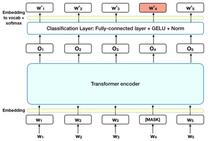
BERT is a transformer encoder, outputing a sequence of the same length as the input sequence.

We randomly mask some tokens with either a special token or some random tokens. We then aim to train the model to minimize the cross entropy between the output and the ground truth. During training, we aim to update parameters of both the BERT and the linear model.

Next Sentence Prediction

This task tries to train the model to output a “yes” for thinking that sentence 2 does follow sentence 1 and a “no” for thinking that sentence 2 does not follow sentence 1. However, this approach is not very useful probably because this task is relatively easy and the model does not learn very much. An alternative way is to use SOP, which trains the model to learn whether sentence 1 is before sentence 2 or after sentence 2.

Fine-tuning

With self-supervised learning, we pre-train the model, which prepares the model for downstream tasks (tasks we care and tasks that we’ve prepared a little bit labeled data). We can then fine-tune the model for different tasks.

With a combination of unlabelled and labelled dataset, this training is called semi-supervised learning.

GLUE

GLUE has $9$ tasks. We fine-tune $9$ models based on the fine-tuned BERT, each for one task below, and then evaluate the model’s performance.

Sequence to Class

Example: sentiment analysis

Note that here, we only randomly initialize the parameters in the linear model, instead of BERT. Also, it’s important that we train the model with labelled dataset.

Fining tuning the model can accelerate the optimization process and improve the performance (lower the loss), as shown in the graph below.

Sequence to Sequence (Same Length)

Example: POS tagging

Two Sequences to Class

Example: Natural Language Inference (NLI)

Extraction-Based Question Answering (QA)

In this case, as usual, both $D$ and $Q$ are sequences of vectors. Both $d_i$ and $q_i$ are words (vectors). In QA system, $D$ is the article and $Q$ is the question. The outputs are two positive integers $s$ and $e$. This means that the answer is in the range from the $s$-th word to the $e$-th word.

The orange and blue vectors are the only two set of parameters we need to train.

Pre-Train Seq2seq Models

It’s also possible to pre-train a seq2seq model. We can corrupt the input to the Encoder and let the Decoder reconstruct the original input.

There’re many ways you can use to corrupt the input.

Why Does BERT work?

The tokens with similar meaning have similar embedding. BERT can output token vectors that represent similar words with high cosine similarity.

There was a similar work conducted called CBOW word embedding. Using deep learning, BERT appeas to perform better. It can learn the contextualized word embedding.

However, learning context of a word may not be the whole story. You can even use BERT to classify meaningless sentences. For example, you can replace parts of a DNA sequence with a random word so that a whole DNA sequence becomes a sentence. You can even use BERT to classify the DNA sequences represented with sentences. Similar works have been done on protein, DNA and music classification.

Multi-Lingual BERT

BERT can also be trained on many languages.

Cross-Lingual Alignment: assign similar embeddings to the same words from different languages.

Mean Reciprocal Rank (MRR): Higher MRR, better alignment

GPT

GPT uses a different pre-training method – next token prediction.

4/22 Lecture 8: Auto-encoder / Anomaly Detection

Auto-encoder

Auto-encoder is often used for dimension reduction (the output vector of the NN encoder). This idea is very similar to Cycle GAN.

The variation of pictures is very limited. There are many possible $n \times n$ matrix. But only a very small subset of them are meaningful pictures. So, the job of the encoder is to make complex things simpler. As seen from the graph below, we can represent the possible pictures with a $1\times2$ vector.

De-noising Auto-encoder

BERT can actually be seen as a de-nosing auto-encoder. Note that the decoder does not have to be a linear model.

Feature Disentanglement

The embedding includes information of different aspects.

However, we don’t need know exactly what dimensions of an embedding contains a particular aspect of information.

Related papers:

Application: Voice Conversion

Discrete Latent Representation

In the last example, be constraining the embedding to be one-hot, the encoder is able to learn a classification problem (unsupervised learning).

The most famous example is: Vector Quantized Variational Auto-encoder (VQVAE).

The parameters we learn in VQVAE are: Encoder, Decoder, the $5$ vectors in the Codebook

This process is very similar to attention. We can think of the output of the Encoder as the Query, the Codebook as Values and Keys.

This method constrains the input of the Decoder to be one of the inputs in the Codebook.

Using this method on speech, the model can learn phonetic information which is represented by the Codebook.

Text as Representation

We can achieve unsupervised summarization using the architecture above (actually it’s just a CycleGAN model). We only need crawled documents to train the model.

Both the Encoder and the Decoder should use seq2seq models because they accept sequence as input and output. The Discriminator makes sure the summary is readable. This is called a seq2seq2seq auto-encoder.

Generator

We can also gain a generator by using the trained Decoder in auto-encoder.

With some modification, we have variational auto-encoder (VAE).

Compression

The image reconstruction is not $100$%. So, there may be a “lossy” effect on the final reconstructed image.

Anomaly Detection

Anomaly Detection: Given a set of training data $\{x^1, x^2, ..., x^N\}$, detecting input $x$​​ is similar to training data or not

Use cases:

Anomaly Detection is better than training a binary classifier because we often don’t have the dataset of anomaly (oftentimes we humans can’t even detect anomaly ourselves). Our dataset is primarily composed of “normal” data. Anomaly Detection is often called one-class classification.

This is how we implement anomaly detecter:

There are many ways we can implement anomaly detection, besides anomaly detecter.

4/29 Lecture 9: Explainable AI

Explainable ML

Interpretable v.s. Powerful

Some models are intrinsically interpretable.

• For example, linear model (from weights, you know the importance of features)
• But not very powerful
• Deep network is difficult to be interpretable. Deep networks are black boxes, but powerful than a linear model.

For a cat classifier:

Local Explanation: why do you think this image is a cat?

Global Explanation: what does a cat look like? (not referring to a specific image)

Local Explanation

For an object $x$ (image, text, etc), it can be composed of multiple components: $\{x_1, ..., x_n, ..., x_N\}$. For each $x_i$ in image it can represent pixel, segment, etc. For each $x_i$ in text, it can represent a word.

We asks the question: “which component is critical for making a decision?” We can therefore remove or modify the components. The important components are those that result in large decision change.

Saliency Map

Sometimes, our Saliency Map may appear noisy (noisy gradient). We can use SmoothGrad to solve that – Randomly add noises to the input image, get saliency maps of the noisy images, and average them.

Integrated Gradient (IG)

However, there may be problems with gradient saturation. Gradients can not always reflect importance. In this case, a longer trunk size does not make the object more elephant. We can use Integrated Gradient to solve this problem.

Network Visualization

We can learn that the network knows that the same sentence spoken by different speaker is similar (erase the identity of the speaker).

Network Probing

Using this method, we can tell whether the embeddings have information of POS properties by evaluating the accuracy of the POS (Part of Speech) or NER (Named-Entity Recognition) classifier. If the accuracy is high, then the embeddings do contain those information.

If the classifier itself has very high bias, then we can not really tell whether the embeddings have those information based on accuracy.

We can also train a TTS model that takes the output of a particular hidden layer as input. If the TTS model outputs an audio sequence that has no speaker information. Then, we can conclude that the model has learned to earse speaker information when doing audio-to-text tasks.

Global Explanation

We can know based on feature maps (the output of a filter) what patterns a particular filter is responsible for detecting. As a result, for an unknown image $X$, we can try to create an image that tries to create a large value of sum in a feature map:

$$ X^* = \arg \max_X \sum_i \sum_j a_{ij} $$

$X^*$ is the image that contains the patterns filter 1 can detect. We can find $X^*$ using gradient ascent. One example of the resulting $X^*$ looks like this:

However, if we try to find the best image (that maximizes the classification probability),

$$ X^* = \arg \max_X y_i $$

we fail to see any meaningful pattern:

The images should look like a digit. As a result, we need to add constraints $R(X)$ – how likely $X$ is a digit:

$$ X^* = \arg \max_X y_i + R(X) $$

where:

$$ R(X) = - \sum_{i,j} |X_{i,j}| $$

$R(X)$ restricts image $X$ to have as little pattern (white regions) as possible since an image of a digit should have a couple of patterns (the rest of the image should just be the cover).

To make the images clearer, we may need several regularization terms, and hyperparameter tuning…

For example, we can append an image generator $G$ (GAN, VAE, etc) before the classifier that we want to understand.

$$ z^* = \arg \max_z y_i $$

We can then get the image we want by calculating:

$$ X^* = G(z^*) $$

Outlook

We can use an interpretable model (linear model) to mimic the behavior of an uninterpretable model, e.g. NN (not the complete behavior, only “local range”).

This idea is called Local Interpretable Model-Agnostic Explanations (LIME)

5/06 Lecture 10: Attack

Adversarial Attack

Example of Attack

White Box Attack

Assume we know the parameters $\boldsymbol{\theta}$ of the Network.

Our goal is to find a new picture $\boldsymbol{x}$ that correspond to an output $\boldsymbol{y}$ that is most different from the true label (one-hot) $\boldsymbol{\hat{y}}$.

Since we also want the noise to be as little as possible, we add an additional constraint: $d(\boldsymbol{x^0}, \boldsymbol{x}) \leq \epsilon$. $\epsilon$​ is a threshold such that we want the noise to be unable to be perceived by humans.

$$ \boldsymbol{x^*} = \arg \min_{\boldsymbol{x}, d(\boldsymbol{x^0}, \boldsymbol{x}) \leq \epsilon} L(\boldsymbol{x}) $$

We also define $\boldsymbol{\Delta x}$: $$ \boldsymbol{\Delta x} = \boldsymbol{x} - \boldsymbol{x^0} $$ This can be seen as: $$ \begin{bmatrix} \Delta x_1 \\ \Delta x_2 \\ \Delta x_3 \\ \vdots \end{bmatrix} = \begin{bmatrix} x_1 \\ x_2 \\ x_3 \\ \vdots \end{bmatrix} - \begin{bmatrix} x_1^0 \\ x_2^0 \\ x_3^0 \\ \vdots \end{bmatrix} $$ There are many ways to calculate distance $d$​ between the two images:

L2-norm: $$ d(\boldsymbol{x^0}, \boldsymbol{x}) = \|\boldsymbol{\Delta x}\|_2 = \sqrt{(\Delta x_1)^2 + (\Delta x_2)^2 + \dots} $$ L-infinity: $$ d(\boldsymbol{x^0}, \boldsymbol{x}) = \|\boldsymbol{\Delta x}\|_{\infty} = \max\{|\Delta x_1|,|\Delta x_2|, \dots\} $$ L-infinity is a better metric for images because it fits human perception of image differences (as seen from the example below). We may need to use other metrics depending on our domain knowledge.

The Loss function can be defined depending on the specific attack:

Non-Targeted Attack:

The Loss function $L$ is defined to be the negative cross entropy between the true label and the output label. Since we want to minimize $L$, this is the same as maximizing $ e(\boldsymbol{y}, \boldsymbol{\hat{y}}) $.

$$ L(\boldsymbol{x}) = - e(\boldsymbol{y}, \boldsymbol{\hat{y}}) $$

Targeted Attack:

Since we want to minimize the Loss function, we add the cross entropy between the output and the target label (since we want the two to be similar, therefore a smaller $e$).

$$ L(\boldsymbol{x}) = - e(\boldsymbol{y}, \boldsymbol{\hat{y}}) + e(\boldsymbol{y}, \boldsymbol{y^{\text{target}}}) $$

How can we do optimization?

If we assume we don’t have the constraint on $\min$, it’s the same as the previous NN training, except that we now update input, not parameters (because parameters are now constant).

1. Start from the original image $\boldsymbol{x^0}$
2. From $t=1$ to $T$: $\boldsymbol{x^t} \leftarrow \boldsymbol{x^{t-1}} - \eta \boldsymbol{g}$​

If we consider the constraint, the process is very similar:

1. Start from the original image $\boldsymbol{x^0}$
2. From $t=1$ to $T$: $\boldsymbol{x^t} \leftarrow \boldsymbol{x^{t-1}} - \eta \boldsymbol{g}$​​
3. If $d(\boldsymbol{x^0}, \boldsymbol{x}) > \epsilon$, then $\boldsymbol{x^t} \leftarrow fix(\boldsymbol{x^t})$​

If we are using L-infinity, we can fix $\boldsymbol{x^t}$ by finding a point within the constraint that is the closest to $\boldsymbol{x^t}$.

FGSM

We can use Fast Gradient Sign Method (FGSM, https://arxiv.org/abs/1412.6572):

Redefine $\boldsymbol{g}$ as: $$ \mathbf{g} = \begin{bmatrix} \text{sign}\left(\frac{\partial L}{\partial x_1} \bigg|_{\mathbf{x}=\mathbf{x}^{t-1}}\right) \\ \text{sign}\left(\frac{\partial L}{\partial x_2} \bigg|_{\mathbf{x}=\mathbf{x}^{t-1}} \right) \\ \vdots \end{bmatrix} $$ Here, each entry is either $1$ or $-1$: if $t>0$, $\text{sign}(t) = 1$; otherwise, $\text{sign}(t) = -1$.

1. Start from the original image $\boldsymbol{x^0}$
2. Do only one shot: $\boldsymbol{x^t} \leftarrow \boldsymbol{x^{t-1}} - \epsilon \boldsymbol{g}$​​

In the case of L-infinity, $\boldsymbol{x}$ will move to either of the four corners.

There’s also an iterative version of FGSM, which is basically doing Step 2 $T$​ iterations

Black Box Attack

What if we don’t have parameters of a private network?

If you have the training data of the target network:

1. Train a proxy network yourself
2. Using the proxy network to generate attacked objects

If we don’t have training data, we can just the targeted network to generate a lot of data points.

It’s also possible to do One Pixel Attack (only add noise to one pixel of an image) and Universal Adversarial Attack (use one noise signals to attack all the image inputs for a model).

Attack in Physical World

• An attacker would need to find perturbations that generalize beyond a single image.
• Extreme differences between adjacent pixels in the perturbation are unlikely to be accurately captured by cameras.
• It is desirable to craft perturbations that are comprised mostly of colors reproducible by the printer

Adversarial Reprogramming

“Backdoor” in Model

• Attack happens in the training phase
• We need to be careful of open public dataset

Passive Defense

Passive Defense means that we do not change the parameter of the model.

The overall objective is to apply a filter to make the attack signal less powerful.

One way to implement this is that we can apply Smoothing on the input image. This will alter the attack signal, making it much less harmful. However, we need to pay attention to its side effect – it may make the classification confidence lower, though it rarely affects the accuracy.

We can also use image compression and generator to implement this.

However, these methods have some drawbacks. For example, if the attackers know these methods are used as defenses, they can obtain a signal that has taken into account these filters (just treat them as the starting layers of the network). Therefore, we can use randomization.

Proactive Defense

We can use Adversarial Training (training a model that is robust to adversarial attack). This method is an example of Data Augumentation.

Given training set $\mathcal{X} = \{(\boldsymbol{x^1}, \hat{y}^1), ..., (\boldsymbol{x^N}, \hat{y}^N)\}$:

Using $\mathcal{X}$​ to train your model

1. For $n = 1$ to $N$: Find adversarial input $\boldsymbol{\tilde{x}^n}$ given $\boldsymbol{x^n}$​ by an attack algorithm

2. We then have new training data $\mathcal{X}' = \{(\boldsymbol{\tilde{x}^1}, \hat{y}^1), ..., (\boldsymbol{\tilde{x}^N}, \hat{y}^N)\}$

3. Using both $\mathcal{X}$ and $\mathcal{X}'$​​ to update your model

4. Repeat Steps 1-3

However, if we did not consider an attack algorithm in Adversarial Training, this method will not prevent the attack from that algorithm.

However, Adversarial Training is very computationally expensive.

5/13 Lecture 11: Adaptation

Domain Adaptation

Domain shift: Training and testing data have different distributions

There are also many different aspects of doman shift:

If we have some labeled data points from the target domain, we can train a model by source data, then fine-tune the model by target data. However, since there’s only limited target data, we need to be careful about overfitting.

However, the most common scenairo is that we often have large amount of unlabeled target data.

We can train a Feature Extractor (a NN) to output the features of the input.

Domain Adversarial Training

Domain Classifier is a binary classifier. The goal of the Label Predictor is to be as accurate as possible on Source Domain images. The goal of the Domain Classifier is to be as accurate as possible on any image.

Domain Generalization

If we do not know anything about the target domain, then the problem we are dealing with is Domain Generalization.

5/20 Lecture 12: Reinforcement Learning

RL

Just like ML, RL is also looking for a function, the Actor.

Policy Network

The Actor architecture can be anything: FC NN, CNN, transformer…

Input of NN: the observation of machine represented as a vector or a matrix

Output of NN: each action corresponds to a neuron in output layer (they represent the probability of the action the Actor will take – we don’t always take the action with maximum probability)

Loss

An episode is the whole process from the first observation $s_1$​ to game over.

The total reward, a.k.a. return, is what we want to maximize:

$$ R = \sum_{t=1}^T r_t $$

Optimization

A trajectory $\tau$ is the set of all the observations and actions.

$$ \tau = \{s_1, a_1, s_2, a_2, ...\} $$

Reward is a function of $s_i$ and $a_i$, the current observation and the current action.

This idea is similar to GAN. The Actor is like a Generator; the Reward and the Environment together are like the Discriminator. However, in RL, the Reward and the Environment are not NN. This makes the problem not able to be solved by gradient descent.

Control an Actor

Make an Actor take or don’t take a specific action $\hat{a}$ given specific observation $s$.

By defining the loss and the labels, we can achieve the following goal:

This is almost like supervised learning. We can train the Actor by getting a dataset:

We can also redefine the loss by introducing weights for each {observation, action} pair. For example, we are more desired to see $\hat{a}_1$ followed by $s_1$ than $\hat{a}_3$ followed by $s_3$.

$$ L = \sum A_n e_n $$

The difficulty is what determines $A_i$ and what $\{s_i, \hat{a}_i\}$ pairs to generate.

Version 0

We can start with a randomly-initialized Actor and then run it with many episodes. This will help collect us with some data. If we see a observation-action pair that produces positive reward, we will assign a positive $A_i$​ value to that pair.

However, generally speaking, this is not a very good strategy since actions are not independent.

• An action affects the subsequent observations and thus subsequent rewards.
• Reward delay: Actor has to sacrifice immediate reward to gain more long-term reward.
• In space invader, only “fire” yields positive reward, so vision 0 will learn an actor that always “fire”.

Version 1

We need to take into account all the rewards that we gain after performing one action at timestamp $t$. Therefore, we can define a cumulated reward (as opposed to an immediate reward in the last version) $G_t$:

$$ A_t = G_t = \sum_{n=t}^N r_n $$

Version 2

However, if the sequence of length $N$ is very long, then $r_N$ if probably not the credit of $a_1$. Therefore, we can redefine $G_t'$ using a discount factor $\gamma < 1$:

Discounted Cumulated Reward: $$ A_t = G_t' = \sum_{n=t}^N \gamma^{n-t} r_n $$

Version 3

But good or bad rewards are “relative.” If all the $r_n \geq 10$, then having a reward of $10$ is actually very bad. We can redefine $A_i$ values by minusing by a baseline $b$. This makes $A_i$ to have positive and negative values.

$$ A_t = G_t' - b $$

Policy Gradient

1. Initialize Actor NN parameters $\theta^0$
2. For training iteration $i=1$ to $T$:
   • Using Actor $\theta^{i-1}$ to interact with the environment.
   • We then obtain data/training set $\{s_1, a_1\}, \{s_2, a_2\}, ..., \{s_N, a_N\}$​. Note that here the data collection is in the for loop of training iterations.
   • Compute $A_1, A_2, ..., A_N$
   • Compute Loss $L=\sum_n A_n e_n$
   • Update Actor parameters using gradient descent: $\theta^i \leftarrow \theta^{i-1} - \eta \nabla L$​

This process (from 2.1 to 2.3) is very expensive. Each time you update the model parameters, you need to collect the whole training set again. However, this process is necessary because it is based on the experience of Actor $\theta^{i-1}$。 We need to use a the new Actor $\theta^i$​’s trajectory to train the new Actor.

On-Policy Learning: the actor to train and the actor for interacting are the same.

Off-Policy Learning: the actor to train and the actor for interacting are different. In this way, we don’t have to collect data after each update

• One example is Proximal Policy Optimization (PPO). The actor to train has to know its difference with the actor to interact.

Exploration: The actor needs to have some randomness during data collection (remember that we sample our action). If the initial setting of the actor is always performing one action, then we will never know whether other actions are good or bad. If we don’t have randomness, we can’t really train the actor. With exploration, we can collect more diverse data. We sometimes want to even deliberately add randomness. We can enlarge output entropy or add noises onto parameters of the actor.

Critic

Critic: Given actor $\theta$, how good it is when observing $s$ (and taking action $a$​).

• An example is value function $V^{\theta}(s)$: When using actor $\theta$, the discounted cumulated reward (see Version 2) expected to be obtained after seeing $s$. Note that since the function depends on $\theta$, the same observation $s$ will have a different associated value if the actors are different. The output values of a critic depend on the actor evaluated.

MC & TD

How to train a critic?

One way is to use Monte-Carlo (MC) based approach: The critic watches actor $\theta$ to interact with the environment. However, we can only update $V^{\theta}$ after the episode is over.

$V^{\theta}(s_a)$ should be as close as possible to $G'_a$ and $V^{\theta}(s_b)$ should be as close as possible to $G'_b$.

Another way is Temporal-difference (TD) approach. We don’t need to wait for the entire episode.

MC and TD may produce different results for the same $V^{\theta}$​ with the same dataset as seen from the following example in Sutton v2 (Example 6.4).

That is because MC and TD have different assumptions. For TD, we assume that $s_a$ can not influence $s_b$ (no correlation). It is possible that our dataset (the samples) is limited. For MC, we assume that $s_a$ can influence $s_b$. It is possible that observing $s_a$ influences the reward of observing $s_b$ so that it is always zero.

Version 3.5

How can we use critic on training actor?

Recall that in Version 3, we introduce a baseline $b$ as normalization. How to choose $b$? One possible way is to set $b = V^{\theta}(s_t)$. $$ A_t = G_t' - V^{\theta}(s_t) $$

Why this method works? Remember that $V^{\theta}(s_t)$ takes into account many episodes, so it’s an expected value. This makes $A_t$ very intuitive.

Version 4: Advantage Actor-Critic

However, Version 3 is still problematic because $G_t'$ may be very random (it’s just a sample). It may be very good or bad. We want it to resemble an average value like $V^{\theta}(s_t)$​​​.

Therefore, for a pair $\{ s_t, a_t \}$: $$ A_t = \left[r_t + V^{\theta}(s_{t+1})\right] - V^{\theta}(s_t) $$ Note that $s_{t+1}$ is the observation of the environment influenced by the actor taking action $a_t$.

The parameters of actor and critic can be shared. In practice, the first several layers are shared in common. If the observation is an image, then the convolutional layers will be shared.

Reward Shaping

In tasks like robot arm bolting on the screws, the reward $r_t$ is always or mostly $0$​ (spare reward) because the actor is randomly initialized and it will very likely fail to complete the task. So, we may not know what actions are good or bad. As a consequence, developers can define extra rewards to guide agents. This is called reward shaping.

For example, we can incentive the actor to do different things by defining extra rewards based on our domain knowledge.

We can also add curiosity as an extra reward: obtaining extra reward when the agent sees something new (but meaningful).

Imitation Learning

Defining a reward can be challenging in some tasks. Hand-crafted rewards can lead to uncontrolled behavior.

We can use Imitation Learning. We assume that actor can interact with the environment, but reward function is not available.

We can record demonstration of an expert (for example recording of human drivers in self-driving cars training). We define $\{\hat{\tau}_1, ..., \hat{\tau}_K\}$, where each $\hat{\tau}_i$​​ is one trajectory of the expert. Isn’t this supervised learning? Yes, this is known as Behavior Cloning. This method has several problems:

• The experts only sample limited observation. The actor will not know what to do in other edge cases.
• The agent will copy every behavior, even irrelevant actions.

Inverse RL (IRL)

This is vanilla RL:

Inverse RL has the exact opposite direction of process. It first learns the reward function and then uses that reward function to find the optimal actor.

The principle is that the teacher is always the best. As a result, the basic algorithm is:

1. Initialize an actor.

2. In each iteration:

   1. The actor interacts with the environments to obtain some trajectories.
   2. Define a reward function, which makes the trajectories of the teacher better than the actor.
   3. The actor learns to maximize the reward based on the new reward function.
   4. Repeat.

3. Output the reward function and the actor learned from the reward function.

IRL is very similar to GAN:

5/27 Lecture 13: Network Compression

Preparation 1: Network Pruning and Lottery Ticket Hypothesis

We may need to deploy ML models in resource-constrained environments because of lower-latency and privacy concerns.

NN are typically over-parameterized – there’s significant redundant weights or neurons.

How to evaluate the importance of a weight? We can either look at its absolute value or its $b_i$​ value as seen in life-long learning.

How to evaluate the importance of a neuron? We can record the number of times it didn’t output a $0$​ on a given dataset.

After pruning, the accuracy will drop (hopefully not too much). We can then fine-tune on training data for recover. Remember not to prune too much at once, or the NN won’t recover. We can do the whole process iteratively.

Weight pruning is not always a very effective method. The network architecture becomes irregular (not fully-connected anymore). It also becomes harder to implement and harder to speed up (if you set the pruned weights to $0$, then you are not actually making the NN any smaller).

Neuron pruning is a better method as it helps the NN architecture stay regular. It’s also easy to implement and easy to speedup.

How about simply train a smaller network?

It is widely known that smaller network is more difficult to learn successfully. It is easier to first train a large NN and then gradually reduce its size.

The Lottery Ticket Hypothesis states that a large network is like a bunch of sub-networks so that we have a higher chance of train the network successfully.

Preparation 2: Other ways

Knowledge Distillation

There are two NNs: one large Teacher Net, one small Student Net.

The Student Net can hopefully learn the information that “1” is similar to “7” from the output of the Teacher Net. This is better than simply learning from the dataset labels. In practice, we may also use an ensemble NN to represent the Teacher Net.

We may add Temperature for softmax $T$, a hyperparameter, when doing Knowledge Distillation:

$$ y_i' = \frac{\exp{\frac{y_i}{T}}}{\sum_j \exp{\frac{y_j}{T}}} $$

The temperature can help make sharp distribution a little bit smoother. This is critical because vanilla softmax can produce results very similar to the one-hot label in the dataset.

Parameter Quantization

Less Bits

We can use less bits to represent a value (lowering the numerical precision).

Weight Clustering

Huffman encoding

We can represent frequent clusters by less bits, represent rare clusters by more bits.

Binary Weights

It’s even possible to make your weights always $+1$ or $-1$​. One classical example is Binary Connect.

Architecture Design: Depthwise Seperable Convolution

Depthwise Convolution

Depthwise convolution considers the interaction within a specific channel.

The filter number must be equal to the input channel number (each filter only considers one channel). The number of input channels must be equal to the number of output channels. The filters are $k \times k$ matrices.

However, one problem is that there is no interaction between channels.

Pointwise Convolution

Pointwise convolution considers the interaction amongst channels.

The filter number does not have to be equal to the input channel number. However, we force the filter size to be $1 \times 1$.

Number of Parameters Comparison

Since $O$ is usually a very large number, we can safely ignore $\frac{1}{O}$. Therefore, the standard CNN uses $k^2$ times more parameters than Depthwise Seperable Convolution.

Low rank approximation

$$ M = WN=U(VN)=(UV)N $$

Therefore, we can approximate the matrix $W=UV$ though there’re some constraints on $W$ (it’s low-rank).

The Depthwise Seperable Convolution is very similar to this idea of using two layers to replace one layer in order to reduce the parameter size.

6/03 Lecture 14: Life-Long Learning

Preparation 1: Catastrophic Forgetting

Challenges

Life-Long Learning (LLL) is also known as Continuous Learning, Never Ending Learning or Incremental Learning.

This problem is also evident in real-world applications:

One example of the problem LLL tries to tackle is:

The network has enough capacity to learn both tasks. However, it still failed.

It’s not because machine are not able to do it, but it just didn’t do it.

Even though multi-task training can solve this problem, this may lead to issues concerning computation and storage. For example, if we want to train the model on the dataset of the 1000-th task, we have to store the previous 999 tasks. However, multi-task training can be considered as the upper bound of LLL.

Training a model for each task is also a possible solution. However, we cannot store all the models obviously for storage reasons. More importantly, this way, knowledge cannot transfer across different tasks.

Live-Long v.s. Transfer

LLL is different from transfer learning. In transfer learning, we don’t care about whether the model can still do the old task.

Evaluation

Here, $R_{i,j}$ means the performance (accuracy) on task $j$ after training task $i$​.

• If $i>j$, after training on task $i$, does the model forgot task $j$?
• If $i

We can define the accuracy to be:

$$ \text{score} = \frac{1}{T} \sum_{i=1}^{T} R_{T,i} $$

Alternatively, we can define the accuracy using a metric called Backward Transfer:

$$ \text{score} = \frac{1}{T-1} \sum_{i=1}^{T-1} R_{T,i} - R_{i,i} $$

Since $R_{T,i}$ is usually smaller than $R_{i,i}$, the score is usually negative.

We are also interested in the knowledge transfer. Therefore, there’s another score metric called Forward Transfer:

$$ \text{score} = \frac{1}{T-1} \sum_{i=2}^{T} R_{i-1,i} - R_{0,i} $$

Preparation 2: Solutions

Selective Synaptic Plasticity

This is a regularization-based approach.

Here is a clear visualization explaining why Catastrophic Forgetting would occur.

The basic idea of Selective Synaptic Plasticity is that some parameters in the model are important to the previous tasks. We shall only change the unimportant parameters.

We can revise the loss function that we want to minimize.

$$ L'(\boldsymbol{\theta}) = L(\boldsymbol{\theta}) + \lambda \sum_i b_i (\theta_i - \theta_{i}^{b})^2 $$

Each parameter learned from the previous tasks $\theta_i^b$ has a “guard” $b_i$ representing how important the parameter is to the previous tasks. $\theta_i$ is the parameter to be learning. $L(\boldsymbol{\theta})$ is the loss for current task.

• If $b_i=0$, there’s no constraint on $\theta_i$. This will lead to Catastrophic Forgetting.
• If $b_i = \infty$, $\theta_i$ would always be equal to $\theta_i^b$​. This will prevent the model from learning anything from training, leading to Intransigence.

We humans set the values of $b_i$. Different papers have talked about different ways to calculate the value of $b_i$.

There’s also an older method called Gradient Episodic Memory (GEM):

The learning order also plays a role in whether Catastrophic Forgetting occurs. Thus we have Curriculum Learning:

6/10 Lecture 15: Meta Learning

Meta Learning

We can define $\phi$, the learnable components of the learning algorithm $F_{\phi}$. For example, in DL, $\phi$ may include NN architecture, initial parameters, learning rate, etc.

We also need to define loss function $L(\phi)$ for learning algorithm $F_{\phi}$. We need support of different tasks to conduct meta learning. This is often called Across-Task Training, whereas the vanilla machine learning is called Within-Task Training.

How do we evaluate the loss? We can evaluate the classifier on the testing set. Note that training examples (often called support set) and testing examples (often called query set) here are both in the training task.

The loss $l^i$ is the sum of cross entropy for each datapoint. We can then define our total loss $L(\phi) = \sum_{i=1}^{N} l^i$, where $N$​ is the number of training tasks. We can then find the optimal $\phi^* = \arg \min_{\phi} L(\phi)$​​.

Here, the loss of meta learning is different from ML:

Using the optimization approach, if you know how to compute $\frac{\partial L(\phi)}{\partial \phi}$, gradient descent is your friend. What if $L(\phi)$ is not differentiable (for example, $\phi$ is a discrete value such as the number of layers in the network)? We can use Reinforcement Learning or Evolutionary Algorithm. We can therefore get a learned “learning algorithm” $F_{\phi^*}$.

In typical ML, you compute the loss based on training examples. In meta learning, you compute the loss based on testing examples.

The general framework of meta learning looks like this:

Note that in the testing time, meta learning is different from vanilla ML as it uses Across-Task Testing. The process of one Within-Task Training and one Within-Task Testing is called one episode.

Across-Task Training is often called the outer loop and Within-Task Training is often called the inner loop.

Meta learning is often used to achieve one-shot learning – we only need a few examples to train a network if the learning algorithm is good enough.

Machine learning is about finding a function $f$. Meta learning is about finding a function $F$ that finds a function $f$​.

What you know about ML can usually apply to meta learning:

• Overfitting on training tasks
• Get more training tasks to improve performance
• Task augmentation
• There are also hyperparameters when learning a learning algorithm (But hopefully, we can obtain an optimal learning algorithm that can be applied on future tasks)
• Development tasks, alongside training tasks and testing tasks (just like development set used in ML)

Recalled the gradient descent algorithm:

We can learn the initialized parameter $\boldsymbol{\theta}$ (this idea is in MAML).